Overview

The Java Queue<E> interface declares the interface for the Queue data structure. A number of JCF classes implement this interface. In this assignment you will make use of the queue data structure and the Jaffe-Smith algorithm (described below) to synthesize the sound a guitar makes when one of its strings is plucked.

About Sounds

The fundamental tone of a musical note is represented by a sine wave at a specific frequency. The table below gives the frequencies of different notes in the diatonic (common) scale.

Note: The # symbol following the above letters (e.g. A#) means "A-sharp". On a piano, the "sharps" are the black keys. In modern music (which employs something called "equal temperament"), A-sharp is the same note as B-flat, C-sharp is the same as D-flat, and so on, but this was not always the case. Early keyboard instruments actually divided the black keys into two parts that produced slightly different tones!

Doubling the frequency gives you the same note one octave higher while halving the frequency gives you the same note one octave lower.

Sending a sinusoidal waveform with the appropriate frequency to your computer's speakers will generate the desired tone. The play() method from the SimpleAudio class accepts a ''List'' of floating point values and sends them to the computer's speakers.

In order to do this, we need to chose how often to send a value to the speakers. This is known as the sampling rate and typically is in the range of 8,000 to 48,000 samples per second. If we wished to hear the note middle C for a quarter of a second at 8,000 samples per second, we would need to generate a sequence of 2,000 samples (if we need 8,000 samples for one second of sound, a quarter second of sound will require a quarter of 8,000 (i.e., 2,000 samples)).

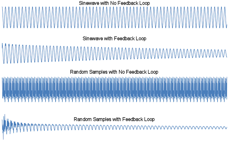
The samples should be such that they produce a sinusoidal waveform that repeats its sinewave 262 Hz (times per second). Therefore, our 2,000 samples will describe a periodic sinewave that completes 65.5 cycles (262/4). Such a waveform can be seen in the first plot below. If you were to listen to this sound, it would be the "hum" a tuning fork makes when it is struck. The second plot is this sound //decaying// (getting softer or dying away) over time.

Sound waveforms

Jaffe-Smith Algorithm

The Jaffe-Smith algorithm makes use of a queue data structure to generate a waveform that simulates the sound made by plucking a string on a guitar. The waveform of a guitar plucking sound is not purely sinusoidal - it is more complex, but still periodic. The Jaffe-Smith algorithm needs to know the duration of the sound, the desired frequency of the simulated guitar string, the sampling rate, and something called the decay rate (which controls how quickly the sound fades to silence).

To begin, you must initialize an empty List<Float> instance, samples, that will hold the waveform generated by the Jaffe-Smith algorithm.

Then for each note in the Guitar object, the following must be done:

Initialization Phase

The algorithm begins by:

1. Calculating the number of samples per period, samplesPerPeriod, as the sampling rate divided by the desired frequency.
2. Calculating the number of samples, numberOfSamples, as the sampling rate multiplied by the duration of the sound. Keep in mind that the sampling rate is in units of samples per second and the duration is in units of milliseconds.
3. Initialize a Queue<Float>. This queue, periodSamples, is populated with samplesPerPeriod random floating point values between -1.0 and 1.0. Don't worry about why for now, we'll get to that later.
4. A variable called previousSample is initialized to zero.

At this point, the periodSamples queue contains one period of the sound waveform.

Looping Phase

If the periodSamples queue contained one period of a 262 Hz sinusoidal waveform, it would be easy to generate 65.5 cycles of the waveform (like in the example above) by looping numberOfSamples times where each time through the loop we would take the sample off the front of the queue, add it to the back of the samples list and also add it to the back of the periodSamples queue. In the process of doing this, we would have copied one cycle of the sinusoid into the samples list 65.5 times.

However, instead of just adding the samples from the periodSamples queue onto the back of the samples list, the algorithm calculates a new sample value by multiplying the decayRate by the average of the current sample and previousSample.

The looping phase begins with an empty samples list and ends with a full samples list. The loop runs numberOfSamples times and each time through the loop the following are done:

1. Dequeue the current sample off of the periodSamples queue.
2. Calculate the new sample value as the product of the decay rate and the average of the previous sample and current sample.
3. The new sample value is enqueued on the periodSamples queue and added to the samples list.
4. The previousSample variable is given the value of the current sample. (Note: the current sample is the value that was dequeued at the beginning of the loop, not the newly calculated value.)

Once the looping phase has completed, the samples list contains all of the samples to be sent to the speakers.

Jaffe-Smith Algorithm Intuition

It is not critical to understand the algorithm in order to complete the lab assignment; however, a brief (and simplified) description follows.

The periodSamples queue stores one complete period of the waveform to be repeated. As discussed previously, if the periodSamples queue stored one cycle of a sinusoidal wave, then a waveform representing a note of a given frequency and duration could be generated by just making multiple copies of the samples found in the periodSamples queue.

The Jaffe-Smith algorithm does two things differently:

1. The samples stored in the periodSamples queue are random in nature instead of a nice sinusoidal wave.
2. The samples are modified slightly each time through the queue.

Randomized Starting Point for periodSamples

At first glance it may seem rather odd to use a bunch of random values as the starting point for the periodic waveform since the random nature of the values may generate additional frequencies within; however, consider the initial pluck of a guitar string. A guitar pluck begins with an abrupt plucking of a string followed by a duration of time when the string "finds" its resonate frequency, i.e., the frequency at which it likes to vibrate. Immediately after the guitar string has been plucked, it is not vibrating at its resonate frequency. Therefore, it does not seem unreasonable to begin with random values.

If we were to eliminate the second change made by the Jaffe-Smith algorithm, the waveform would still produce the desired note, but the sound would be distorted. The third waveform in graph above, titled "Random Samples with No Feedback Loop" shows an example of such a waveform.

Feedback Loop

The second thing that the Jaffe-Smith algorithm does is modify the value of each sample slightly each time the sample is encountered again. There are essentially two things going on here: 1) the amplitude of the waveform is gradually reduced by the decay rate (set to 0.99 for the example graphs above); and 2) the waveform is becoming smoother as a result of the current sample being averaged with the previous sample.

The averaging with the previous value makes the curve smoother because two neighbors that have similar values retain their similar value while two neighbors that have significantly different values are brought closer to the middle value by the averaging process. The averaging process also serves to further reduce the amplitude of the waveform since the magnitude of the result of averaging two numbers is never more than the maximum of the two numbers (and that only happens if both numbers are equal, which is highly unlikely). The magnitude reduction is most pronounced when the two numbers being averaged are least alike, i.e., if the two numbers being averaged are equal, then no change occurs; however, if one is 1.0 and the other is -1.0, the average is 0.0.

The second plot, entitled "Sinewave with Feedback Loop," shows how the amplitude of the waveform diminishes over time. Since the waveform was very smooth to begin with, the averaging process does not exhibit any smoothing. In contrast, the fourth plot, entitled "Random Samples with Feedback Loop," clearly demonstrates the smoothing affect of the averaging process. The amplitude of the waveform experiences a more rapid reduction since the neighbors that are being averaged together may not have similar values.

This is an example of something called Digital Signal Processing. By writing this algorithm, you're implementing one kind of Digital Signal Processor that synthesizes a guitar pluck sound. Commercial musical synthesizers implement many other variations of Digital Signal Processors as well.

Assignment Details

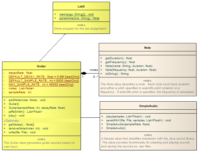
Your assignment is to write a program that will read in one or more notes specified in a text file and use the Jaffe-Smith algorithm to simulate the sequence of notes being plucked on a guitar. You will be working with the four classes shown in the following UML class diagram:

Class Diagram

The SimpleAudio and Note classes have already been written for you. You should not modify these files. You will complete the implementation of two classes: Lab5 and Guitar. You can find documentation describing how each class should function by following the links to the Javadoc. Note that three of the methods in the Guitar class are marked as optional. You are not required to implement these methods.

Your program must be able to read text files in the following format. Each line in the file should consist of at least two fields. The first field specifies the pitch of the note using scientific pitch notation. The second field specifies the duration of the note in milliseconds (could be a floating point number). Each field must be separated by whitespace. Any additional text on a line in the file should be ignored. Blank lines are allowed in the file and should be ignored by your program.

If a line in the file does not conform to the above requirements, your program should display a warning message indicating that the line was ignored and then continue to the next line. Your program should not crash (terminate due to an exception being thrown).

An example input file is shown below:

G4 312.5 // Deck
F4 125 // the
E4 250 // halls
D4 250 // with
C4 250 // boughs
D4 250 // of
E4 250 // hol
C4 250 // ly

D4 125 // Fa
E4 125 // la
F4 125 // la
D4 125 // la
E4 312.5 // la
D4 125 // la
C4 250 // la
B3 250 // la
C4 500 // la

The files needed for this project are available in this .zip file.

Acknowledgements

This assignment was written by Dr. Chris Taylor.

Lab Deliverables